Technological results

Particle synthesis
Dynamic convolution

References

The third basic goal of the T-EMP project was to: “further develop music technological tools motivated by issues encountered through the artistic work in the ensemble, including music software for artistic performance and sound synthesis. The development work is closely tied to developing a new repertoire and new forms of artistic expression for the ensemble T-EMP. We wish to make these development projects open and available for the interested public.”

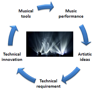
Technological development in T-EMP is closely tied to artistic needs

The project’s strongest technological contributions have been made to support the concept of live processing, which allows members of the ensemble to process sounds from each other in a real-time performance situation. The Method chapter has already introduced this concept along with the two processing techniques that we have focused our attention on: granular synthesis and convolution. Both have received considerable innovative contributions from the project, predominantly in the form of freely available music software. In addition to this, we have also started experimenting with live interprocessing, a paradigm where two live input signals directly affect each other. This enables a three-way performative network of interactions, where one musician controls the processing of two signal generating musicians, and the signal of these two affect each other in various ways. Interprocessing can be enabled by live streaming convolution (described more below), but it can also be explored with other processing techniques. The area of interprocessing has barely been touched upon in the current project but is seen as a promising field for further research.

Our preferred platform for software experimentation and development is the open source, platform-independent computer music software Csound [1]. Csound was initially developed in the mid-1980s by Barry Vercoe at MIT. Over the years it has grown through a collaborative effort into a very powerful system for music programming. Today is has a highly efficient audio engine, a huge collection of open-source audio processing functions, and a very active community of contributors and users. We write our software tools in the Csound language itself or implement them as opcodes extending the language [2]. Furthermore, the tools are made available as audio plugins with graphical user-interfaces, to allow ease of use and integration in standard music applications. The plugins are either generated with the Cabbage tool, or programmed from scratch as custom plugin wrappers around the Csound instrument. All code is open and freely available, and the tools themselves can be downloaded free of charge.

The following two sections,  Particle synthesis and Dynamic convolution, will give further details on the processing tools we have developed, including references to published papers. Granular synthesis is referred to as particle synthesis, as the latter term also incorporates a number of techniques derived from granular synthesis. Furthermore we use the term dynamic convolution to highlight that responsiveness and dynamic control play particularly important roles in our convolution experiments.

back to top

Particle synthesis

Our work on granular synthesis has matured over a long time. The foundation was laid by Øyvind Brandtsegg during his artistic research project on musical improvisation with computers [4], finished in 2008. Under his supervision a very powerful granular synthesizer named partikkel was developed by NTNU master students Thom Johansen and Torgeir Strand Henriksen [5]. The name hints to the term “particle synthesis” which we use to cover granular synthesis and all its variations, similar to usage found in Curtis Roads’ seminal book “Microsound” [6].

Since partikkel has a large number of parameters it can be unwieldy to control in a live performance situation. We’ve augmented the synthesizer with a dynamic mapping matrix that actually extends its functionality with a large number of modulation and effect operators, for a total of over 200 real-time controllable parameters [7]. In order to ease the utilization of all this expressive power in performance, we provided an interpolation mechanism to navigate between matrix states. For the nontechnical reader, the notion of matrix states of a musical instrument may seem somewhat unfamiliar. For more discussion on the practical purpose of mapping, see the chapter on Control Intimacy.

We launched the Hadron particle synthesizer [8] as a freely available audio plugin supporting the VST and AU plugin standards in November 2011.The plugin provides user interaction with partikkel and the modulation matrix through a user-friendly GUI containing a simple XY-pad that allows navigation between four predefined matrix states [9]. This instrument has been very well received by the interested public. It plays a significant role in the T-EMP setup, and is actively used by Øyvind, Bernt Isak and Tone. Design of processing routines in the form of Hadron states was an integral part of the development in the current research project, as was the practical exploration of the (custom states of the) instrument as used for live sampling and processing .

Granular synthesis and its varieties

We presented the partikkel opcode at the Linux Audio Conference 2011 [10]. A summary of the paper will be given in the following. With the intent of showing why granular synthesis is a very flexible tool for live improvised sound processing, we start out with presenting the granular synthesis technique and a number of its known varieties. All of them are available through our granular synthesizer.

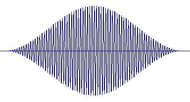
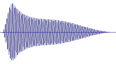
The building block of granular synthesis is the grain, a brief microacoustic event with duration near the threshold of human hearing, typically in the range 1 to 100 milliseconds [4]. The figure above shows a typical grain: a sinusoidal waveform shaped by a Gaussian envelope. Typical control parameters are:

• Source audio: arbitrary waveform (sampled or periodic). In T-EMP we commonly use live sampled sources or simply use a buffered live input stream.

• Grain shape: envelope function for each grain   

• Grain duration   

• Grain pitch: playback rate of source audio inside the grain

The global organization of grains introduces one more parameter:

• Grain rate: the number of grains per second

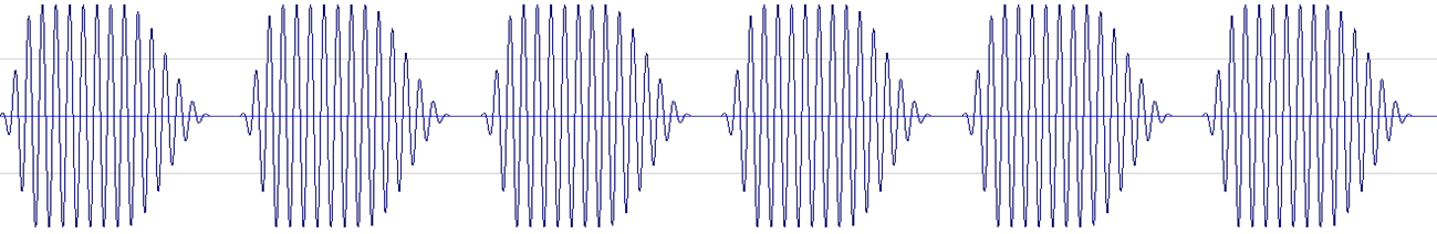
In synchronous granular synthesis, the grains are distributed at regular intervals as shown in the figure above. For asynchronous granular synthesis the grain intervals are irregularly distributed, and in this case it might be more correct to use the term grain density than grain rate. The concept of a granular cloud is typically associated with asynchronous grain generation within specified frequency limits. The latter can easily be controlled from outside the grain generator by providing a randomly varied, band-limited grain pitch variable.

A number of varieties of granular synthesis are integrated into partikkel by expanding the basic parameter set:

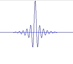
Glisson synthesis is a straightforward extension of basic granular synthesis in which the grain has an independent frequency trajectory [6]. The grain or glisson creates a short glissando (see figure above). In order to meet this requirement the granular generator must allow specification of both start and end frequency for each individual particle and also allow control over the pitch sweep curve (the rate of progression from starting pitch to ending pitch).

Grainlet synthesis is inspired by ideas from wavelet synthesis. We understand a wavelet to be a short segment of a signal, always encapsulating a constant number of cycles. Hence the duration of a wavelet is always inversely proportional to the frequency of the waveform inside it. Duration and frequency are linked (through an inverse relationship). Grainlet synthesis is based on a generalization of the linkage between different synthesis parameters. Grainlet synthesis does not impose additional requirements on the design of the granular generator itself, but suggests the possibility of linking parameters, which can conveniently be accomplished in a control structure external to the actual granular audio generator unit.

Trainlet synthesis. The specific property that characterizes a trainlet (and also gives rise to its name) is the audio waveform inside each grain. The waveform consists of a band-limited impulse train as shown in the figure above. The trainlet waveform has to be synthesized in real time to allow for parametric control over the impulse train. This dictates that the trainlet must be considered a special case when compared to single cycle or sampled waveforms used in the other varieties of particle synthesis.

Pulsar synthesis introduces two new concepts to our universal particle synthesis engine: duty cycle and masking. Here the term pulsar is used to describe a sound particle consisting of an arbitrary waveform (the pulsaret) followed by a silent interval. The total duration of the pulsar is labeled the pulsar period, while the duration of the pulsaret is labeled the duty cycle. A feature associated with pulsar synthesis is the phenomenon of masking. This refers to the separate processing of individual pulsar grains, most commonly by applying different amplitude gains to each pulsaret (see the figure above for an example). To be able to synthesize pulsars in a flexible manner, we enabled functionality for grain masking of a wide range of parameters (amplitude, output routing, source waveform mix, pitch transposition and frequency modulation) in our general granular synthesizer.

Formant synthesis. Granular techniques are commonly used to create a spectrum with controllable formants, for example to simulate vocals or speech. Several variants of particle-based formant synthesis (FOF, Vosim, Window Function Synthesis) have been proposed [6]. Formant wave-function (FOF) synthesis requires separate control of grain attack and decay durations, and commonly uses an exponential decay shape (see the figure above). These requirements are met in the design of our all-including granular generator.

As we have already pointed out, the generator supports arbitrary waveforms within the grains. As a matter of fact the grain waveform is a distinguishing characteristic of several granular varieties. In order to morph between them the particle generator must support gradual transitions from one waveform to another. The waveform might also be a live input, effectively turning the particle synthesizer into a live processing effect.

One important reason for designing an all-including particle generator is to enable dynamic interpolation between the different varieties. The musician should not only be able to pick a particular granular variety, but actually move seamlessly between them to explore intermediate states. This includes gradually transforming the very role of the particle synthesizer from signal source to signal processor.

Mapping and the modulation matrix

Our mapping strategy, and in particular the modulation matrix has enabled us to use the complex particle synthesis generator performatively as a musical instrument. The modulation matrix was presented at the NIME conference in May 2011 [7]. A summary is presented here:

Digital musical instruments allow us to completely separate the performance interface from the sound generator. The connection between the two is what we refer to as mapping. Several researchers have pointed out that the expressiveness of digital musical instruments really depends upon the mapping used, and that creativity and playability are greatly influenced by a mapping that motivates exploration of the instrument (see e.g. [9]). In fact, experiments presented by Hunt et al [11] indicate that “complex mappings can provide quantifiable performance benefits and improved interface expressiveness”. Rather than simple one-to-one parameter mappings between controller and sound generator, complex many-to-many mappings seem to promote a more holistic approach to the instrument: “less thinking, more playing”. We will elaborate these issues in chapter on Control intimacy.

The importance of efficient mapping strategies becomes obvious when controlling sound generators with a large number of input parameters in a live performance context. An interesting strategy proposed by Momeni and Wessel employs geometric models to characterize and control musical material [12]. They argue that high-dimensional sound representations can be efficiently controlled by low-dimensional geometric models that fit well with standard controllers such as joysticks and tablets. Typically a small number of desirable sounds are represented as high-dimensional parameter vectors (e.g. the parameter set of a synthesis algorithm) and associated with specific coordinates in two-dimensional gesture space. When navigating through gesture space new sounds are generated as a result of an interpolation between the original parameter vectors. Spatial positions can easily be stored and recalled as presets, and the gesture trajectories lend themselves naturally to automation.

We have adopted their strategy in our Hadron particle synthesizer to facilitate user control over more than 200 synthesis, modulation and effect parameters. The parameter vector not only represents a specific sound, but also contains information on how manual expression controllers and internal modulators may influence the sound. As a result, navigation in gesture space actually modifies the mapping and hence changes the instrument itself.

The key mechanism for integrating this rich behavior into the mapping is the dynamic modulation matrix. The general idea is to regard all control parameters as modulators of the sound generator, and to do all mapping in one single matrix. The modulation matrix defines the interrelations between modulation sources and synthesis parameters in a very flexible fashion, and also allows modulation feedback. The entire matrix is dynamically changed through interpolation when the performer navigates gesture space.

The origin of the modulation matrix is found in the patch bays of old analogue synthesizers, where patch cords interconnected the various synthesizer modules. The concept is still common in software synthesizers and plug-ins. Software-based matrix modulation typically includes a list of modulation sources, a list of modulation destinations, and “slots” for each possible connection between source and destination. As an extension of the straightforward routing in classic patch bays software matrices often provide two controls between modulation source and destination:

• Scaling coefficient: The amount of modulation source reaching the destination.

• Initial value: An initial, fixed modulation value.

Our implementation of the modulation matrix is available as a Csound opcode with the name modmatrix [13]. The opcode computes a table of output values (destinations) as a function of initial values, modulation variables and scaling coefficients. The i’th output value is computed as:

outi=ini+kgkimk

where outi is the output value, ini is the corresponding initial value, mk is the k’th modulation variable and gki is the scaling coefficient relating the k’th modulation variable to the i’th output.

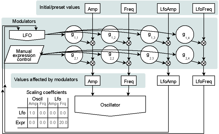
The figure above shows a simple example of a modulation matrix with 4 parameters and 2 modulators. The modulators are a low frequency oscillator (LFO) and a manual expression controller (for direct user interaction). The parameters are amplitude and frequency of an output signal oscillator and amplitude and frequency of the modulating LFO itself. As some of the parameters are used in the synthesis of modulator signals, we have modulator feedback. Modulator feedback implies that some modulation sources may take the role as modulation destinations as well and we get self-modifying behavior controlled by the modulation matrix. As with any other kind of feedback, modulator feedback must be applied with caution.

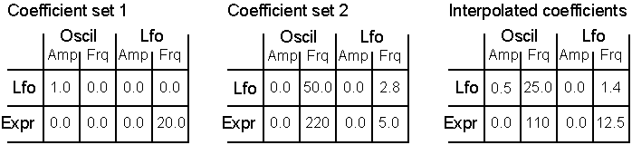
Since the scaling coefficients are stored in a table, we can dynamically alter the mapping in the modulation matrix by manipulating the values in the coefficient table. We can of course explicitly write values to the table, but more interesting: we can interpolate between different mapping tables. The three tables above shows how this could work: The first two tables represent two predefined coefficient sets. If we interpolate between them, the midway position would look equal to the third table. Interpolation of modulation matrices (coefficient sets) is the key to enable mapping between gesture space (user control) and the instruments parameter space.

Hadron Particle Synthesizer

Hadron Particle Synthesizer is a complex granular synthesis device built around the Csound opcodes partikkel and modmatrix. It is freely available for download both as a Max for Live device and as a VST/AU plugin. A simplified control structure was developed to allow real-time performance with precise control over the large parameter set using just a few user interface controls (see screenhot of graphical interface (GUI) above). The modulation matrix is essential to link simplicity of control to the complexity of the parameter set in this instrument. Compared to the modulation matrix involved in Hadron, the matrix example discussed in the previous section is trivial, but still representative.

Hadron allows mixing of 4 source waveforms inside each grain, with independent pitch and phase for each source. The source waveforms can be recorded sounds or live audio input. The grain rate and pitch can be varied continuously at audio rate to allow for frequency modulation effects, and displacement of individual grains allows smooth transitions between synchronous and asynchronous granular techniques. To enable separate processing of individual grains, a grain masking system is incorporated, enabling “per grain” specification of output routing, amplitude, pitch glissandi and more. A set of internal audio effects (ring modulators, filters, delays) may be applied for further processing of individual grains.

The Hadron Particle Synthesizer also utilizes a set of modulators (modulation sources) for automation of parameter values. The modulators are well known signal generators, such as low frequency oscillators (LFO), envelope generators and random generators. In addition, audio analysis data (amplitude, pitch, transients) for the source waveforms may be used as modulator signals as well. Within Hadron, any signal that can affect a parameter value is considered a modulator, including the signals from MIDI note input and the 4 manual expression controls (see GUI above). There is also a set of programmable modulator transform functions to allow waveshaping, division, multiplication and modulo operations on (or of) modulator signals.

The full parameter set for Hadron currently counts 209 parameters and 51 modulators. The granular processing requires “only” about 40 of these parameters, and a similar amount of parameters are used for effects control. The largest chunk of parameters is actually the modulator controls (e.g. LFO amplitude, LFO frequency, envelope attack, etc.) with approximately 100 parameters.

Hadron makes use of a state interpolation system similar to the techniques suggested by Momeni and Wessel [12], but in our case the parameter vector represents not only a specific sound, but also contains information on how manual expression controllers and internal modulators may influence the sound. As a result navigation in gesture space actually modifies the mapping and hence changes the instrument itself. This means that the effect of e.g. an LFO or a manual expression controller can change gradually from one state to another.  It is also possible to let one expression controller affect the mapping of another via scaling and transfer functions. Through this dynamic mapping scheme we expand the degrees of freedom beyond the number of controls exposed.

The main performance controls provided by the Hadron user interface (see picture above) are a two-dimensional (2D) control pad for interpolating between instrument states and four expression controls. The expression controls have no specific label, since their effect may change radically as the performer navigates between the different states. The four corners of the 2D pad refer to pre-designed states representing specific coordinates in the N-dimensional synthesis parameter space, and the pad provides navigation along an elastic surface spanned by these four coordinates.

At any given point the four expression controls constitute what we can call the “reachable parameter space” with four degrees of freedom. This does not necessarily mean that the reachable parameter space has only four dimensions, since each expression control may be (possibly non-linearly) mapped to more than one parameter. Taken together the 2D pad and the expression controls represent 6 degrees of freedom for movement within the N-dimensional parameter space. This constitutes a significant simplification, making the space more manageable for a user. Still, the dynamic mapping and the ability to change origin, scale and orientation of the axes imposes complexity that may confuse the user.

Our technological exploration of granular synthesis has definitely reached a mature level with the Hadron instrument. The next issue is playability: To what extent does Hadron facilitate musical expressivity in a live performance context? The instrument poses new challenges with respect to the musician’s intellectual and intuitive understanding of it since the semantics of the external control parameters may change during performance. This leads to a change of focus from technical concerns to listening and intuitive action.

To be able to perform fluently and expressively with this instrument, is seems essential that the user spends considerable time getting familiar with the reachable parameter space. At first glance, this may seem as an unnecessary complex situation. Why not just extract a few commonly used parameters and create a simple mapping with labeled controls? Here we may draw a parallel to the situation encountered when learning to play a traditional acoustic instrument. With a traditional acoustic instrument there are typically a number of physical parameters (e.g. bow pressure and string tension on a violin) that affect several aspects of the sound produced by the instrument. When learning to play, focus on the details of the sound produced while modifying the playing technique (e.g. where on the string to pluck) is essential in gaining a high control intimacy [14] between performer and instrument. The connection between control and sound is learned intuitively. A similar approach should be encouraged for digital musical instruments.

We presented some user experiences from performing with Hadron at the Forum Acusticum conference June 2011 [15]. The most skilled user is Øyvind Brandtsegg, prime system designer of Hadron. His intimate knowledge of the sound producing functions of the instrument significantly enhances the control intimacy. He also has exclusive access to designing parameter states. That said, his impression is that the control parameter mapping in Hadron gives intuitive access to the many-dimensional parameter space in a clear and concise manner. Indeed, the relationship between control and synthesis parameters is complex and dynamic, and it requires time and practice to become familiar with the instrument. It appears that significantly longer time of familiarisation was needed to perform and improvise live with the instrument compared to compositional use.

Live performance with the instrument has been explored in a duo setting with acoustic percussion, where the acoustic instruments are used as audio input for Hadron. Brandtsegg’s main preparation for these performances was spent on familiarisation with the different Hadron states used. In this process an explorative method was used, to some degree supported by the technical knowledge of both the synthesizer implementation and the details of the parameter set in the state. Some new states were specifically crafted to solve issues encountered in the preparation process. A significant portion of the time spent was used on understanding how the expression controls would actually function when interpolation was performed between the selected states. Even if one knows intimately the detailed settings of each parameter in each state, the space covered when interpolating from state to state is unknown also for the author of the different states.

A number of external users have evaluated Hadron as well, most of them for a relatively short time. Some have explored the instrument in the studio, while others have used it for live performances. A more thorough research project on user responses may be conducted at a later time.

The general impression from the user responses is that they would use the instrument when something “new” or “different” was called for, something interesting that one does not yet know what it is. The instrument also seems to promise a vast amount of variation and sonic diversity. Many of the users would find it a bit “wild” though, especially the interpolation between different states on the XY pad is experienced as providing too coarse control. A common response is that the XY pad provides more dramatic change in the instrument timbre, and that the expression controls are used for fine tuning. However, there is no inherent reason why the 2D pad and the expressions controllers could not be viewed as equally coarse or fine, and that each of these controls just provides a direction of movement around the parameter space.

The concept of interpolation between different types of effects (e.g. interpolation between a flanger and a grain delay) is something that most users are not used to even think about, so it takes some getting used to. However, those who spent more time on familiarisation with the instrument controls did have no problems using it in an improvised manner for live performance. They were specifically asked if the dynamic nature of the instrument controls seemed prohibitive in terms of their willingness to take risks and explore new sounds during live performance with an audience. One of the users responded that “[the controls] are some of the most fun aspects of the system.  The idea of morphing between these 4 "presets" (states) is particularly exciting.” There is still no doubt that the fact that a control may function differently in different contexts, is new to most users. One remarkable and consistent response is that the users describe the controls’ response as “organic”. The perceived organic quality of the controls was heightened when the user connected a physical interface to manipulate the controls.

The absence of functional descriptions for the instrument controls is reported as frustrating at some times, and liberating at others. Exploring the available control space is sometimes perceived as a random hunt, something that is clearly challenging.

The testers were asked if Hadron invites to an “intellectual and analytic” or an “experimental and intuitive” approach and the answers clearly tend towards the latter. The basis for this is the vast potential for variation, combined with the dynamic mapping and the lack of functional labels for the controls. The design of the user interface seems to encourage experimentation. Several users were surprised that granular synthesis could produce these timbres, even if most of them did know the synthesis technique fairly well from beforehand. “Once it is set up... the system is rather intuitive to work with... that doesn't mean that it is clear what is going on in the algorithms” one user says, and goes on: “The instrument rewards both approaches - from the intuitive side there are galaxies of sounds available in the worlds that intersect on the XY space. But one is rewarded once they know more about the algorithms and what is happening under the hood.”

Figuring out which source sounds work best with a specific parameter state is something that might appear slightly confusing to some users. To a certain degree this is by design, as a certain state might be used with considerable success on a source material that it was not designed for. The output sound of the instrument will obviously change significantly depending on the selection of source audio for processing, and this is an aspect where the user can experiment and personalize the instrument.

To conclude: The Hadron Particle Synthesizer is a flexible digital musical instrument with a vast potential for sonic exploration. The early reports from testers indicate that it is a demanding, but highly rewarding instrument to work with. It is designed for active exploration of new, rich sonic territories, both as part of the compositional process and as a responsive tool in a live performance setting. In T-EMP it has been used by several members of the group, as a tool for extensive and free shaping of improvised input streams.

back to top

Dynamic convolution

While Hadron and particle synthesis had reached a mature technological stage when T-EMP was launched, our exploration of convolution had just started to pick up momentum. Trond Engum investigated convolution as part of his artistic research project, finished December 2011 [16]. His investigations were also presented at the NIME conference earlier the same year [17]. A particular focus was the artistic possibilities offered by convolving musical and concrete, real-world sounds. This approach differs from the traditional uses of convolution in electroacoustic music where one of the two inputs is a preallocated impulse response characterizing a reverberant space or a simple, non-recursive filter. When both convolution inputs are spectrally rich signals, the sounding result will combine their characteristics in ways that are hard to predict and control, but with a great potential for timbral innovation.

Engum has focused on the musical rather than technical implications of this technique and has pursued it with three different approaches: Convolution in post-production, real-time convolution and the live sampling convolver. The first two approaches could be executed with existing convolution tools, while the third approach is linked to the development of custom software.

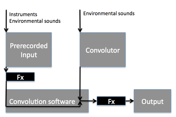
In both the post-production and real-time approach prerecorded environmental sounds were stored as “impulse responses” ( IRs or convolutors) in advance and then applied to a second input as part of convolution experiments. However in post-production the second input is also prerecorded (see figure above) and convolution was applied as a processing effect in a series of empirical investigations aiming to predict how various inputs and IRs would interact with each other.

In post-production there is no way to let the convolution output influence the input. Hence the next natural step was to apply convolution in real-time performance. Using a live input from the performer enables a direct interaction with the output of the convolution process. The musician interacts differently depending on the response he/she gets from the instrument. In fact the sonic behavior of the instrument may change dramatically during convolution, and this will necessarily influence the musician's behavior as well. It makes a big difference to play with short, percussive sounds compared to long, stretched timbres. In order to achieve this two-way communication it was crucial that the musician was separated from the acoustic sound of the instrument in order to interact with the processed signal. This was maintained by feeding back the processed signal to the musician through headphones. The figure below illustrates the feedback mechanism.

Based on the experiences made when investigating real-time convolution, the idea was conceived that we should be able to record and interact with “impulse responses” during live performance. This provides the musician with the opportunity to sample IRs from their own instrument, or more importantly, from other musicians or sound sources, and directly convolve them with another chosen sound-source in real-time. Live sampling convolution opens up for new and exciting ways of interplay within a group of musicians and has become an obvious candidate for further exploration within the context of T-EMP. Unfortunately there are no off-the-shelf convolution tools that support this feature. We had to develop the tools ourselves.

Aim of technological development

There are basically two approaches for implementing the convolution of sound segments, either in the time-domain or in frequency domain. Ideally time-domain convolution has no latency, but the computational costs are prohibiting for segments of any significant length. As an example the convolution of signals of 2 seconds length will typically involve several billion multiplications. Frequency-domain or fast convolution is far more efficient [18]. It does however introduce latency equal to the segment length, which is undesirable for real-time applications. The solution is partitioned convolution which reduces latency by breaking up the input signal into smaller partitions. This is the technique we have extended in our development.

Common to most known applications of convolution is that one of the inputs is a static impulse response (characterizing a filter, an acoustic space or similar), allocated and preprocessed prior to the convolution operation. Impulse responses are typically short and/or with a pronounced amplitude decay throughout its duration. The convolution process does not normally allow parametric real-time control. These are limitations that we wanted to overcome.

We wanted to explore convolution as a creative sound morphing tool, using the spectral and

temporal qualities of one sound to filter another. This is closely related to cross-filtering [19] or cross-synthesis, although in the latter case one usually extracts the spectral envelope of one of the signals prior to their multiplication in the frequency domain [20].

An important aspect of our approach is that both impulse response and input should be dynamically updated during performance. This adds significant amounts of complexity, both with respect to technical implementation and practical use. Without any real-time control of the convolution process, it can be very hard to master in live performance. Depending on the amount of overlap of spectral content between the two signals, the output amplitude may vary by several orders of magnitude. Also, when both input sounds are long, significant blurring may appear in the audio output as the spectrotemporal profiles are layered.

A possible workaround is to convolve only short fragments of the input sounds at a time,

multiplying them frame by frame in the frequency domain. The drawback is that any musically significant temporal structure of the input signals will be lost in the convolution output. To capture the sound's evolution over time requires longer segments, with the possible artifact of time smearing as a byproduct. This seems to be a distinguishing factor in our approach to convolution and cross-synthesis.

The aim of our technological investigations into convolution has been to:

• create dynamic parametric control over the convolution process in order to increase playability

• investigate methods to avoid or control dense and smeared output

• provide the ability to update/change the impulse responses in real-time without glitches

• provide the ability to use two live input sounds to a continuous, real-time convolution process

The motivation behind the investigations is the artistic research within the ensemble T-EMP and specific musical questions posed within that context.

Convolution experiments

The experimental work has produced various digital convolution instruments, for simplicity

called convolvers, using Csound and Cabbage. This work was presented at the Linux Audio Conference 2013 [21]. The experiments can be grouped under two main headings: Dynamic updates of the impulse response, and parametric control of the convolution process.

From our point of view processing with a static impulse response does not fully exploit the

potential of convolution in live performance. We therefore wanted to investigate strategies for dynamically updating the impulse response.

The live sampling convolver

As a first attempt, we implemented a convolver effect where the impulse response could be

recorded and replaced in real-time. This is the idea that spun out of Trond Engum’s research mentioned above. It was intended for use in improvised music performance, similar to traditional live sampling, but using the live recorded audio segment as an impulse response for convolution instead. No care was taken to avoid glitches when replacing the IR in this case, but the instrument can be used as an experimental tool to explore some possibilities.

Input level controls were used to manually shape the overall amplitude envelope of the sampled IR, by fading in and out of the continuous external signal. This proved to be a simple, but valuable method for controlling the timbral output. In our use of this instrument we felt that the result was a bit too static to provide a promising basis for an improvised instrumental practice. Still, with some enhancements in the user interface, such as allowing the user to store, select and re-enable recorded impulse responses, it could be a valuable musical tool in its own right.

The stepwise updated IR buffer

The next step was to dynamically update the impulse response during convolution. A possible (more conventional) application of this technique could be to tune a reverberation IR during real-time performance. A straightforward method to accomplish this without audible artifacts is to use two concurrent convolution processes and crossfade between them when the IR needs to be modified. When combined with live sampling convolution, the crossfade technique renders it possible to do real-time, stepwise updates of the IR, using a live signal as input. In this manner the IR is updated and replaced without glitches, always representing a recent image of the input sound.

The figure above illustrates the concept: Impulse responses are recorded in alternating buffers A and B from one of the inputs. Typical buffer length is between 0.5 and 4 seconds with 2 seconds as the most common. An envelope function is applied to the recorded segments for smoother convolution. The second input is routed to two parallel processing threads where it is convolved with buffer A and B respectively. The convolution with buffer A fades in as soon as that buffer is done recording. Simultaneously the tail of convolution with buffer B is faded out and that buffer starts to record. This allows us to use two live input signals to the convolution process. There is however an inherent delay given by the buffer length. Future research will explore partitioned IR buffer updates to reduce the delay to the length of a single FFT frame.

Signal preprocessing

Convolution can be very hard to control even for a knowledgeable and experienced user [19]. A fundamental goal for our experiments has been to open up convolution by providing enhanced parametric control for real-time exploration of the technique.

As we have noted, the convolution process relates all samples of the IR to all samples of the

input sound. This can easily result in a densely layered, muddy and spectrally unbalanced output. We furnished our convolver with user-controlled filtering (high-pass and low-pass) on both convolution inputs, as this can reduce the problem of dense, muddy output considerably. The point is to provide dynamic control over the “degree of spectral intersection” [20].

The transient convolver

As another strategy for controlling the spectral density of the output, while still keeping with the basic premise that we want to preserve the temporal characteristics of the IR sound, we split both the IR and the input sound into transient and sustained parts. Convolving with an IR that contains only transients will produce a considerably less dense result, while still

preserving the large-scale spectral and temporal evolution of the IR.

The splitting of the transient and sustained parts was done in the time domain by detecting

transients and generating a transient-triggered envelope (see figure above). The transient analysis can be tuned by a number of user-controlled parameters. The sustained part was extracted by using the inverted transient envelope. Hence the sum of the transient and sustained parts are equal to the original input. Transient splitting enables parametric control over the density of the convolution output, allowing the user to mix in as much sustained material as needed. It is also possible to convolve with an IR that has all transients removed, providing a very lush and broad variant.

The various convolution experiments outlined above were combined into a single convolver. It works with two live audio inputs: one is buffered as a stepwise updated IR and the other used as convolution input. The IR can be automatically updated at regular intervals. The sampling and replacement of the IR can also be relegated to manual control, as a way of “holding on” to material that the performer finds musically interesting or particularly effective.

Each of the two input signals can be split into transient and sustained parts, and simple low-pass and high-pass filters are provided as rudimentary methods for controlling spectral spread. Straightforward cross-filtering, continuously multiplying the spectral profile of the two inputs frame by frame, was also added to enable direct comparison and further experimentation. As should be evident from the figure below the user interface provides a great deal of parametric control of this convolver.

In practical use, the effect is still hard to control. This relates to the fact that, with real-time stepwise updates of the IR, the performer does not have detailed control over the IR buffer content. The IR may contain rhythmic material that are offset in time, creating offbeat effects or other irregular rhythmic behavior. With automatic IR updates the performer does not have direct and precise control over the timing of IR changes. Instead the sound of the instrument will change at regular intervals, not necessarily at musically relevant instants.

A possible way of controlling rhythmic consistency would be to update the IR in synchrony with the tempo of the input material, for instance so that the IR always consists of a whole measure or beat and that it is replaced only on beat boundaries. Another proposal would be to strip off non-transient material at the start of the IR, so that the IR would always start with a transient. This leads us to the most recent convolution experiment we have initiated: The live convolver.

The live convolver: cross convolution of two live signals

The live convolver tries to provide the musician with the spectral processing characteristics of convolution while at the same time offer adjustable rhythmic responsiveness and real-time control of temporal smearing through interactive transient detection. The concept of “impulse response” is no longer relevant since both inputs are treated in the same way. The technique was developed in collaboration with master students from the NTNU Acoustics group and will be presented at the 10th International Symposium on Computer Music Multidisciplinary Research (CMMR) in Marseille this year [22].

The live convolver extends the partitioned convolution technique. It splits up the audio segments (typically up to 2 seconds of length) into small blocks and performs blockwise multiplications in the frequency domain. Because the oldest block from the first input is multiplied with the most recent block of the second input, and vice versa, we call this frequency domain cross multiplication (see the figure above). It gives a good balance between computational efficiency and output delay.

One interesting feature of this technique is that the cross multiplication can be carried out in an incremental fashion: It produces output as soon as the first blocks have been buffered and only has contributions from blocks already buffered. The consequence is that we may start a convolution while the segments are still growing, allowing for real-time output with a delay of no more than the number of samples within a small block. Similarly, when the segment size has been reached the initial block pairs of each input may be discarded, and the segments shrink by one block each, until they are both empty and the convolution is complete.

How does this solve the problem of rhythmic responsiveness? By using transient detection to retrigger the convolution process at rhythmically significant points in time. When a transient is detected it marks the border between two convolution segments. The first segment is marked as ended and the blocks within that segment are being discarded one by one until empty, while simultaneously a new segment starts to grow incrementally until the next detected transient. The figure above shows an example of a process where a transient is detected after three blocks have entered. The arrows denote multiplications. Notice that when the segment shrinks block pair 1 exits the process first, followed by block pair 2, and so on. This method has proven to give a good balance between responsiveness and the dense timbral characteristic of convolution. Since convolution segments both grow and shrink gradually, the output will typically be a sum of several overlapping convolution processes. The output is scaled depending on the number of blocks and processes involved.

To avoid unlimited growth a maximum segment length must be defined by the user. This length also helps control the density of the output. With a short segment, one gets output which doesn't depend much on past values, while a longer segment results in slower decay of past samples, and a denser, fuller sound. Rhythmic content is emphasized more with shorter segment sizes.

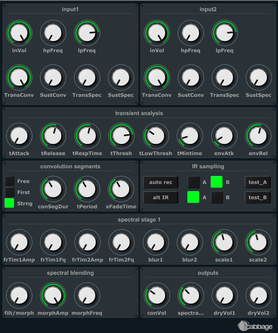
The live convolver has also been implemented as an audio plugin using Csound and Cabbage (see figure above). The parameters controlling the transient detection have a significant impact on the effects behavior. In order to achieve a reasonable level of rhythmic responsiveness the detection sensitivity must be adjusted to pick up only the rhythmically significant transients. The two input channels have independent settings, which makes it possible to do transient detection on one input signal only by clever adjustment of parameters.

To conclude: an algorithm for the live convolution of two continuously changing signals has been  implemented. It offers low output delay, and uses transient detection to segment the signals. It is designed with the intention of being intuitive for musicians to use as well as giving musically meaningful output in a broad range of applications. Parameters which determine how large a portion of the input signals that should contribute to the output have great impact on the spectral density of the output.

We have implemented a number of variations of convolution as an attempt to overcome limitations inherent in convolution as a music processing technique. The context for our experimental work is musical objectives growing out of improvisational practice in electroacoustic music. Preliminary tests show that some of the limitations have been lifted by giving real-time parametric control over the convolution process and the density of its output, and by allowing real-time updates of the IR.

It must be pointed out that the technology is still under development, and that we so far have only limited experience with using these convolution tools in real performance situations. The full musical potential of using convolution within T-EMP remains to be explored. Still, the fruitful dialog between musical needs and technological investigations has proven essential to the project and offers great promise for the future development of both the artistic and the technological aspects of T-EMP.

References:

[1] Csound. See http://www.csounds.com/

[2] V. Lazzarini. 2005. Extensions to the Csound Language: from User-Defined to Plugin Opcodes and Beyond. LAC2005 Proceedings, pages 13.

[3] R. Walsh. 2011. Audio Plugin development with Cabbage. Proceedings of Linux Audio Conference, pages 47-53.

[4] Ø. Brandtsegg. 2008. "New creative possibilities through improvisational use of compositional techniques, - a new computer instrument for the performing musician". Artistic Research project. NTNU. http://oeyvind.teks.no/results/   

[5] Ø. Brandtsegg, T. Johansen, T. Henriksen. The partikkel opcode for Csound. See documentation at: http://www.csounds.com/manual/html/partikkel

[6] Curtis Roads. 2001. Microsound. MIT Press, Cambridge, Massachusetts.

[7] Ø. Brandtsegg, S. Saue, T. Johansen: A modulation matrix for complex parameter sets. In Proceedings of the New Interfaces for Musical Expression Conference (NIME-11), Oslo, Norway, 2011

[8] Ø. Brandtsegg et.al. "The Hadron Particle Synthesizer". www.partikkelaudio.com

[9] Arfib, D., Couturier, J., Kessous, L. and Verfaille, V. Strategies of mapping between model parameters using perceptual spaces. Organised Sound 7, 2 (2002): 127-144

[10] Ø. Brandtsegg, S. Saue, T. Johansen. 2011. Particle synthesis–a unified model for granular synthesis. Proceedings of the 2011 Linux Audio Conference(LAC’11).

[11] Hunt, A., Wanderley, M. and Paradis, M. The importance of parameter mapping in electronic instrument design. Journal of New Music Research 32, 4(2003): 429-440

[12] Momeni, A. and Wessel, D. Characterizing and controlling musical material intuitively with geometric models. In Proceedings of the New Interfaces for Musical Expression Conference (NIME-03) (Montreal, Canada, May 22-24, 2003). Available at http://www.nime.org/2003/onlineproceedings/home.html

[13] Ø. Brandtsegg, T. Johansen. The modmatrix opcode for Csound. See documentation at: http://www.csounds.com/manual/html/modmatrix.html

[14] S. Fels: Designing for intimacy: Creating new interfaces for musical expression. Proceedings of the IEEE 92, 4 (2004)

[15] Ø. Brandtsegg, S. Saue. 2011. Performing and composing with the Hadron Particle Synthesizer. Forum Acusticum, Aalborg, Denmark

[16] T. Engum. 2011. Beat the distance: Music technological strategies for composition and production. Artistic research project. NTNU

[17] T. Engum. 2011. Real-time control and creative convolution. Proceedings of the International Conference on New Interfaces for Musical Expression, pages 519-22.

[18] R. Boulanger, V. Lazzarini. 2010. The Audio Programming Book, The MIT Press

[19] C. Roads. 1997. Sound transformation by convolution. In C. Roads, A. Piccialli, G. D. Poli, S. T. Pope, editors, Musical signal processing, pages 411-38. Swets & Zeitlinger.

[20] Z. Settel, C. Lippe. 1995. Real-time musical applications using frequency domain signal processing. Applications of Signal Processing to Audio and Acoustics, 1995, IEEE ASSP Workshop on, pages 230-3 IEEE.

[21] Ø. Brandtsegg, S. Saue. 2013. Experiments with dynamic convolution techniques in live performance. Proceedings of the 2013 Linux Audio Conference(LAC’13).

[22] L. E. Myhre, A. H. Bardoz, S. Saue, Ø. Brandtsegg, and J. Tro. Cross Convolution of Live Audio Signals for Musical Applications. Accepted paper at the 10th International Symposium on Computer Music Multidisciplinary Research (CMMR) in Marseille, 15-18 October 2013.

back to top