Coordinate change


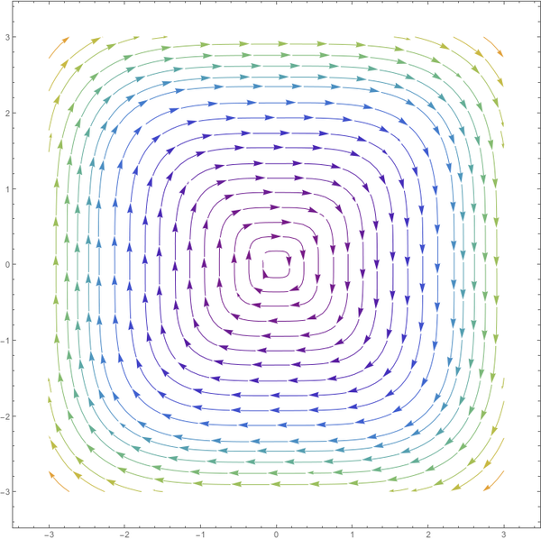
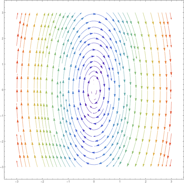
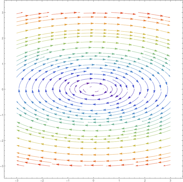
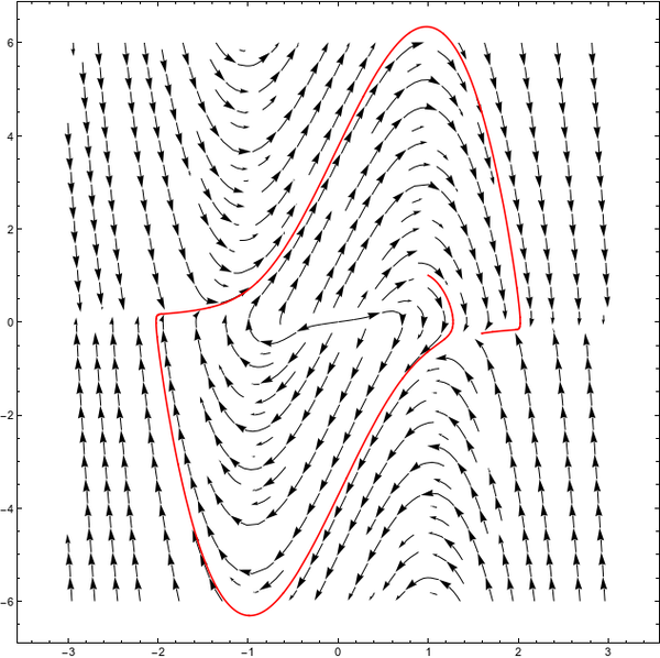
The phase flow of the harmonic oscillator can also be reformulated in a slightly differently. On each radius from the origin, the vector field pushes a point with a constant velocity along a circle. So, we could also say, that the vector field of the harmonic oscillator is a constant on a circle. While, the flow does not "push" in a direction orthogonal to the circle, it does not produce changes in the radius (or amplitude) of the oscillator.


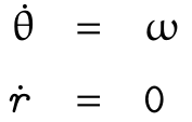
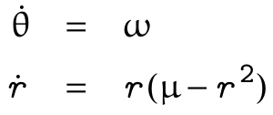
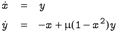
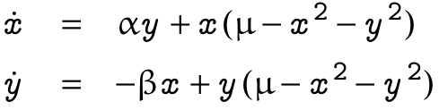
It seems therefore almost natural to reformulate the above equations (in a Cartesian space) in polar coordinates, phase and radius, i.e. an equivalent coordinate space that can highlight the perspective above. We can reformulate the basic harmonic oscillator system as:


The second equation is usually omitted (as clearly it is not so interesting), leaving us with a very concise formulation of oscillatory phenomena. Also, for this reason, as it is done in context of the study of synchronisation phenomena, it is admissible to concentrate on just the differential equation for the phase.


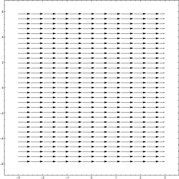
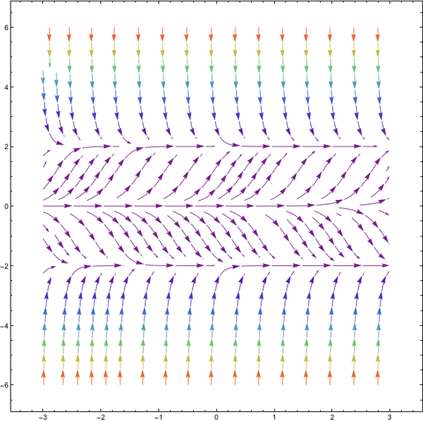
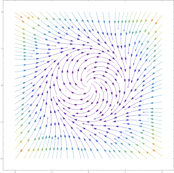
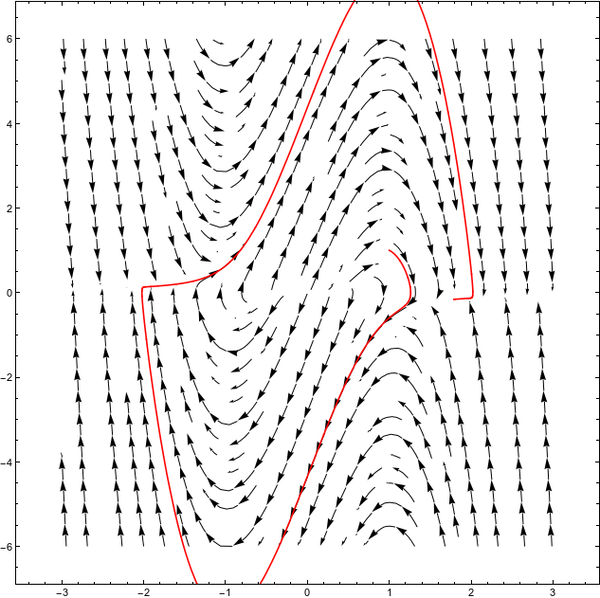
For completeness, note that from the perspective of this coordinate system, also the phase space looks differently (see the figure on the right, the x-axis corresponds to the phase and the y-axis to the radius coordinates). We see a constant of magnitude equal to the frequency of the harmonic oscillator flow directed towards growing values of the phase.


In the theory of dynamical systems, one may encounter many different kinds of oscillators, with many different formulations. Still, reading "through" all these seemingly different equations one can always detect the presence of a similar structure or relationship between the variables involved in the oscillation (usually two). This common structure descends directly from the "godfather" of all oscillators: the harmonic oscillator. Following Hooke's law the harmonic oscillator can be written in the form on the right.

or in the form of ordinary (i.e. first order) differential equations:


Generalising the above formulation, one can see that any system of two differential equations in two variables, of the form on the right with
α and β positive numbers, will produce an oscillatory behaviour. This can be readily seen when looking at the phase space of this system.


The phase space of a particular dynamical system, is the space of all possible states that system can have. Moreover, each point in this space is associated to a vector: the whole space is covered with a vector field. One can image this field as a sort of flow (one speaks of phase flow) that "pushes" each point or state to the next according to the laws of evolution of the system, its differential equations. Fixing a point and following its evolution in time will draw a path in this space which is called a phase trajectory.


For systems as the one above the phase spaces look very similar: in any case, given a starting point, under the influence of the phase flow (depicted as the arrows in the figures on the side) the phase trajectory followed by that point will result in a closed trajectory. In dependence of the relationship between the parameters α and β, it might be a bit stretched in one direction, but the fundamental behaviour, that of returning to the same state from which the observation has begun, is always given. Projecting the motion of the state on one axis will generate a sinusoidal function.


In terms of attractors in this case one speaks of a centre attractor. To note: the only stable point in this phase space, that is a point that remains static for all time, is the origin.


The same behaviour is also given in the case of non-linear equations, like these:
Also in this case, the phase trajectories will result in closed loops around the origin, eve of their form will be a bit more "squarish".


So, the fundamental relationship between variables from which oscillatory behaviour is generated is a relationship that relates the change of one variable to the state of other, with opposite signs for each variable.

Notes on Oscillators


There is a special class of oscillators, which is of particular interest in the phenomena studied under the synchronisation umbrella. These are so-called limit cycles oscillators. Their name refers to the particular form of their associated phase portrait presenting a particular kind of attractor, named in fact limit cycle. A basic formulation for such systems is:


As can be seen from the figure on the right, in this case there is only one closed path, to which all trajectories converge, both from its inside and outside. That is, this oscillator will always tend to oscillate with a given amplitude, determined by the factor μ.


So, the basic "structure" of the oscillation can be read from the above equation, but the addition of the second term in the above equations produces a very different kind of behaviour.


One of the reasons why these systems are of particular interest, is that they are very sturdy, that is very resilient against external perturbations. The centre attractor is instead very weak with respect to perturbation: any disturbance (as for example and dissipation as for example friction) would result in a completely different phase space, system and behaviour, one that is not topologically equivalent to the centre attractor. The limit cycle attractor instead will not produce a qualitatively different behaviour if perturbed by an external force. Probably that is the reason why this kind of systems can be observed in many different natural phenomena and in our body.


A classic example of such oscillator is the van der Pol oscillator:

For μ > 0 this system has a limit cycle which with growing μ grows steeper and steeper.

Coordinate change


In the limit cycle case the change to polar coordinates is a bit different and produces, when applied to the basic form above (not the van der Pol system) a slightly different system.


In this case there is a non-zero component also for the radial part, while the phase changes remain the same as in the canonic harmonic oscillator case. This change expresses the tendency of the system to oscillate but on a circular path of fixed radius
μ.


In the right a plot of the function describing the flow along r. Whenever this function is positive (between 0 and
μ) the flow pushes the radius to grow, while if the function is negative, the flow will pull the radius towards the centre. The overall effect is to drag the radius toward the point in which the value of the flow is 0, the point in which the function crosses the x axis in the graphic.


The phase flow of the above system is depicted on the below.